Beta distribution
Probability density function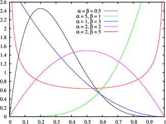 |
|
Cumulative distribution function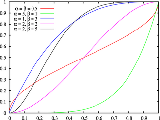 |
|
| parameters: |  shape (real) shape (real) shape (real) shape (real) |
|---|---|
| support: |  |
| pdf: | 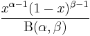 |
| cdf: |  |
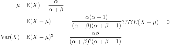
| mean: |  |
| median: |  no closed form no closed form |
| mode: |  for for  |
| variance: |  |
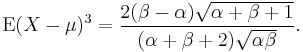
| skewness: |  |
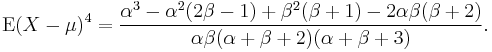
| ex.kurtosis: | see text |
| entropy: | see text |
| mgf: |  |
| cf: |  |
In probability theory and statistics, the beta distribution is a family of continuous probability distributions defined on the interval (0, 1) parameterized by two positive shape parameters, typically denoted by α and β. It is the special case of the Dirichlet distribution with only two parameters. Just as the Dirichlet distribution is the conjugate prior of the multinomial distribution and categorical distribution, the beta distribution is the conjugate prior of the binomial distribution and bernoulli distribution. In Bayesian statistics, it can be seen as the likelihood of the parameter p of a binomial distribution from observing α − 1 independent events with probability p and β − 1 with probability 1 − p.
Contents |
Characterization
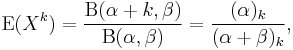
Probability density function
The probability density function of the beta distribution is:
![\begin{align}
f(x;\alpha,\beta) & = \frac{x^{\alpha-1}(1-x)^{\beta-1}}{\int_0^1 u^{\alpha-1} (1-u)^{\beta-1}\, du} \\[6pt]
& = \frac{\Gamma(\alpha+\beta)}{\Gamma(\alpha)\Gamma(\beta)}\, x^{\alpha-1}(1-x)^{\beta-1} \\[6pt]
& = \frac{1}{\mathrm{B}(\alpha,\beta)}\, x
^{\alpha-1}(1-x)^{\beta-1}
\end{align}](/2010-wikipedia_en_wp1-0.8_orig_2010-12/I/b07c588ba27dd60112b7751fac6d77fb.png)
where  is the gamma function. The beta function, B, appears as a normalization constant to ensure that the total probability integrates to unity.
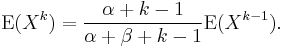
Cumulative distribution function
The cumulative distribution function is
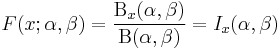
where  is the incomplete beta function and
  is the regularized incomplete beta function.
Properties
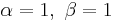
The expected value ( ), first central moment, variance (second central moment), skewness (third central moment), and kurtosis excess (forth central moment) of a Beta distribution random variable X with parameters α and β are:
The skewness is
The kurtosis excess is:
In general, the  th raw moment is given by
where  is a Pochhammer symbol representing rising factorial. It can also be written in a recursive form as
One can also show that

Quantities of information
Given two beta distributed random variables, X ~ Beta(α, β) and Y ~ Beta(α', β'), the information entropy of X is [1]

where  is the digamma function.
The cross entropy is

It follows that the Kullback–Leibler divergence between these two beta distributions is

Shapes
The beta density function can take on different shapes depending on the values of the two parameters:
 is the uniform [0,1] distribution
 is U-shaped (red plot)
 or
or  is strictly decreasing (blue plot)
 is strictly convex
 is a straight line
 is strictly concave
 or
or  is strictly increasing (green plot)
 is strictly convex
 is a straight line
 is strictly concave
 is unimodal (purple & black plots)
Moreover, if  then the density function is symmetric about 1/2 (red & purple plots).
Parameter estimation
Let
be the sample mean and
be the sample variance. The method-of-moments estimates of the parameters are
When the distribution is required over an interval other than [0, 1], say ![\scriptstyle [\ell,h]](/2010-wikipedia_en_wp1-0.8_orig_2010-12/I/6a61ed6e17822a3dea738dd370552cbe.png) , then replace
, then replace  with
with  and
and  with
with  in the above equations.[2][3]
Related distributions
- If X has a beta distribution, then T = X/(1 − X) has a "beta distribution of the second kind", also called the beta prime distribution.
- The connection with the binomial distribution is mentioned below.
- The Beta(1,1) distribution is identical to the standard uniform distribution.
- If X has the Beta(3/2,3/2) distribution and R > 0 is a real parameter, then Y := 2RX – R has the Wigner semicircle distribution.
- If X and Y are independently distributed Gamma(α, θ) and Gamma(β, θ) respectively, then X / (X + Y) is distributed Beta(α, β).
- If X and Y are independently distributed Beta(α,β) and F(2β, 2α) (Snedecor's F distribution with 2β and 2α degrees of freedom), then Pr(X ≤ α/(α + xβ)) = Pr(Y > x) for all x > 0.
- The beta distribution is a special case of the Dirichlet distribution for only two parameters.
- The Kumaraswamy distribution resembles the beta distribution.
- If
![X \sim {\rm U}(0, 1]\,](/2010-wikipedia_en_wp1-0.8_orig_2010-12/I/7487f663a469da4699b115cf58b4ce93.png) has a uniform distribution, then
has a uniform distribution, then  , which is a special case of the Beta distribution called the power-function distribution.
 - Binomial opinions in subjective logic are equivalent to Beta distributions.
- Beta(1/2,1/2) is the Jeffreys prior for a proportion and is equivalent to arcsine distribution.
Beta(i, j) with integer values of i and j is the distribution of the i-th order statistic (the i-th smallest value) of a sample of i + j − 1 independent random variables uniformly distributed between 0 and 1. The cumulative probability from 0 to x is thus the probability that the i-th smallest value is less than x, in other words, it is the probability that at least i of the random variables are less than x, a probability given by summing over the binomial distribution with its p parameter set to x. This shows the intimate connection between the beta distribution and the binomial distribution.
Applications
Rule of succession
A classic application of the beta distribution is the rule of succession, introduced in the 18th century by Pierre-Simon Laplace in the course of treating the sunrise problem. It states that, given s successes in n conditionally independent Bernoulli trials with probability p, that p should be estimated as  . This estimate may be regarded as the expected value of the posterior distribution over p, namely Beta(s + 1, n − s + 1), which is given by Bayes' rule if one assumes a uniform prior over p (i.e., Beta(1, 1)) and then observes that p generated s successes in n trials.
Bayesian statistics
Beta distributions are used extensively in Bayesian statistics, since beta distributions provide a family of conjugate prior distributions for binomial (including Bernoulli) and geometric distributions. The Beta(0,0) distribution is an improper prior and sometimes used to represent ignorance of parameter values.
Task duration modeling
The beta distribution can be used to model events which are constrained to take place within an interval defined by a minimum and maximum value. For this reason, the beta distribution — along with the triangular distribution — is used extensively in PERT, critical path method (CPM) and other project management / control systems to describe the time to completion of a task. In project management, shorthand computations are widely used to estimate the mean and standard deviation of the beta distribution:
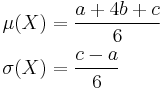
where a is the minimum, c is the maximum, and b is the most likely value.
Using this set of approximations is known as three-point estimation and are exact only for particular values of α and β, specifically when[4]:
or vice versa.
These are notably poor approximations for most other beta distributions exhibiting average errors of 40% in the mean and 549% in the variance[5][6][7]
Information theory
We introduce one exemplary use of beta distribution in information theory, particularly for the information theoretic performance analysis for a communication system. In sensor array systems, the distribution of two vector production is used for the performance estimation in frequent. Assume that s and v are vectors the (M − 1)-dimensional nullspace of h with isotropic i.i.d. where s, v and h are in CM and the elements of h are i.i.d complex Gaussian random values. Then, the production of s and v with absolute of the result |sHv| is beta(1, M − 2) distributed.
Four parameters
A beta distribution with the two shape parameters α and β is supported on the range [0,1]. It is possible to alter the location and scale of the distribution by introducing two further parameters representing the minimum and maximum values of the distribution.[8]
The probability density function of the four parameter beta distribution is given by
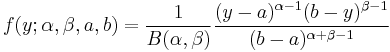
The standard form can be obtained by letting 
References
- ↑ A. C. G. Verdugo Lazo and P. N. Rathie. "On the entropy of continuous probability distributions," IEEE Trans. Inf. Theory, IT-24:120–122,1978.
- ↑ Engineering Statistics Handbook
- ↑ Brighton Webs Ltd. Data & Analysis Services for Industry & Education
- ↑ Grubbs, Frank E. (1962). Attempts to Validate Certain PERT Statistics or ‘Picking on PERT’. Operations Research 10(6), p. 912–915.
- ↑ Keefer, Donald L. and Verdini, William A. (1993). Better Estimation of PERT Activity Time Parameters. Management Science 39(9), p. 1086–1091.
- ↑ Keefer, Donald L. and Bodily, Samuel E. (1983). Three-point Approximations for Continuous Random variables. Management Science 29(5), p. 595–609.
- ↑ DRMI Newsletter, Issue 12, April 8, 2005
- ↑ Beta4 distribution
External links
- Weisstein, Eric W., "Beta Distribution" from MathWorld.
- "Beta Distribution" by Fiona Maclachlan, the Wolfram Demonstrations Project, 2007.
- Beta Distribution – Overview and Example, xycoon.com
- Beta Distribution, brighton-webs.co.uk
- Beta Distributions – Applet showing beta distributions in action.
|
||||||||||||||||||||||||||||||||||||||||||||||||||||||||||||||||||
|
|||||||||||